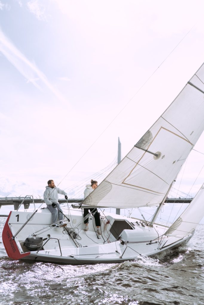
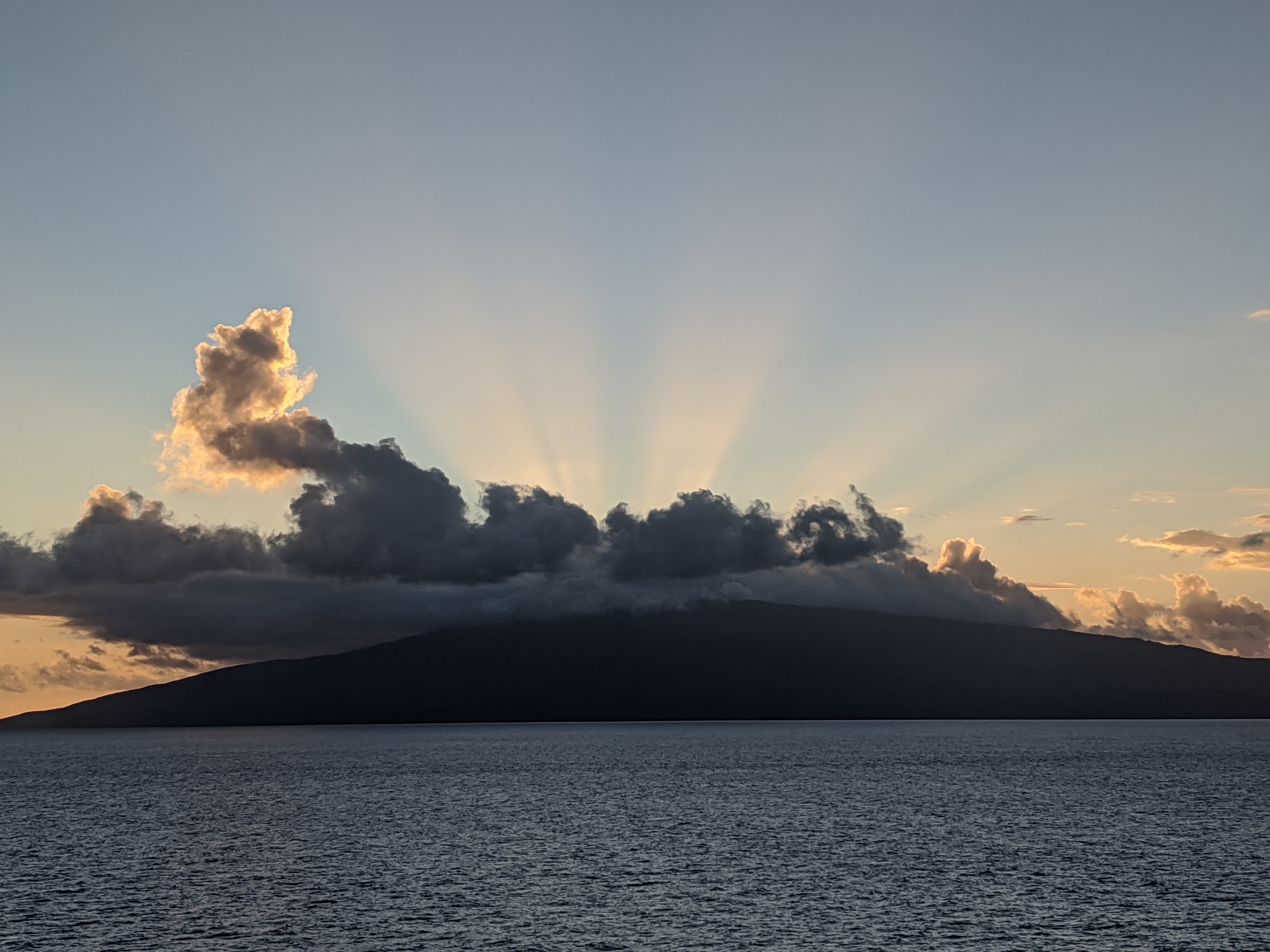
San Francisco Bay is one of the premier sailing areas in the world. What is it that makes the area special?
Easy! The weather. Year round mild conditions allow sailing nearly every day throughout the year. And, consistent 25 to 30 knot winds pretty much every day from May to October have led to a cliché that if you can sail on San Francisco Bay, you can sail anywhere.
Consistent winds
With fog as a downside
The down side? Fog. Interestingly, both conditions are related, and probably would not exist without the other.
It All Starts With:
A high pressure area and a low pressure area and the wind they produce
The impact of wind on water
Something called the coriolis effect
And, finally, the dew point
Add in a mountain range with a single major opening (the Golden Gate) and you have what is arguably the finest sailing in the world!
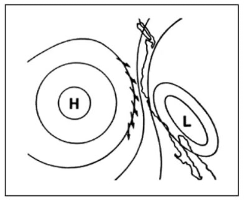
The Wind
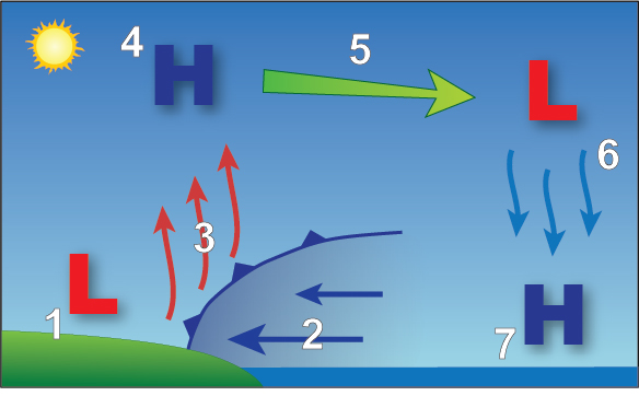
High Pressure to Low Pressure
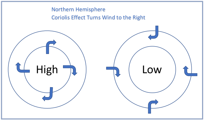
Air flows from higher to lower pressure. The Coriolis Effect caused by the Earth’s rotation turns the air flow clockwise (in the northern hemisphere) around and out of a high pressure system into the lower pressure where it rotates counter clockwise.
Now, visualize that the high pressure is centered over the Pacific Ocean off of San Francisco, and the low pressure over Nevada. San Francisco sits pretty much right in the middle of the two. The resulting wind comes from the north or northwest.
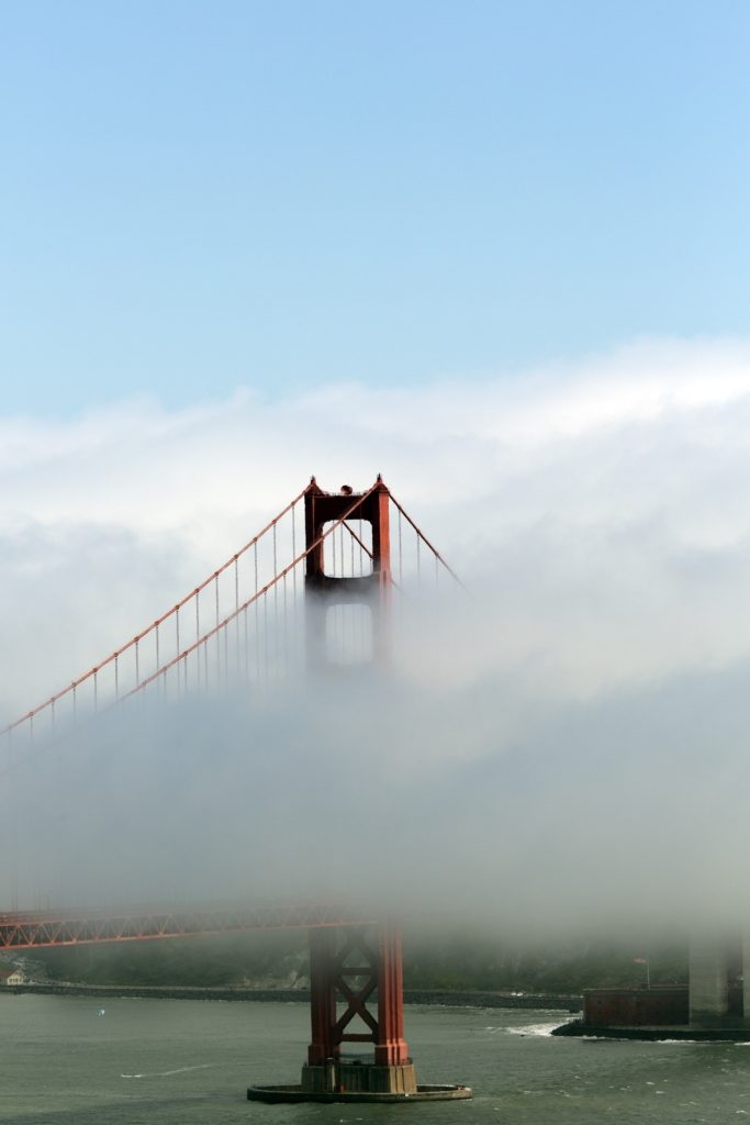
The high pressure air is going to try to fill in the low pressure area, however, the Coast Range of mountains creates a pretty effective barrier. The number one opening through that barrier … The Golden Gate.
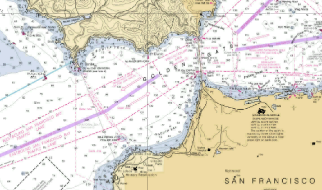
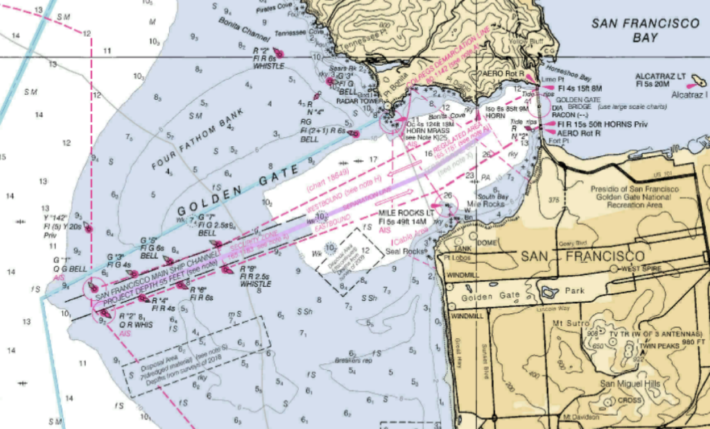
The Golden Gate
2 miles wide at its western opening
Nearly 2.5 miles long
1 mile wide at the entrance into the bay
Oriented from the Southwest to the Northeast, it is the perfect “funnel” to direct and concentrate the wind moving from high into low. From a large area of the Pacific to a small bay.
The Fog
As can be seen in the high/low pressure image, the wind direction off the coast of California is generally north to south.
Steady wind creates current in the water that it passes over. The resulting current in the top few feet of water may be moving to the south with the wind, however, below the surface, the coriolis effect turns that movement to the right about 90 degrees, so that it is moving to the west, away from the coast. The water moving to the west is replaced by very cold water from the depths of the Pacific Ocean.
The air moving across the water is warmer than the water, so, the air gets cooler. When the temperature drops to the level of something called the dew point, moisture in it condenses into fog.
This fog continues to move with the wind and in turn gets “sucked” into the bay resulting in the wind and fog San Francisco is famous for.
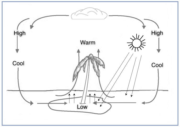
Weather is based on the relationship of the Sun to the Earth.
Warm air rises, cool air sinks, the Earth rotates beneath it, and revolves around the sun.
As simple as it sounds, this sums up the processes driving the weather patterns we experience. We are going to start our weather education looking at a drawing of a large scale process which has been scaled down to size.
In our drawing, rays from the sun pass through the atmosphere to heat the surface of the earth. Land warms more quickly than water.
Warm Air Rises
The warmed land then radiates its heat, warming the air near it. The warm air rises.
Radiation from the sun warms the land, which in turn warms the air around it.
As the warm air rises, it begins to cool back down, and to move away from more new air rising. The cooling continues until eventually the air begins to sink back to the surface where it heads toward the area of rising air, filling in for the air that’s no longer there.
Some important facts
A great deal of information is found in this simple image. Some of it is obvious, and some not.
The sun heats everything, however, land heats faster than water.
Warm air rises. In this case, the “packet” of air directly above the island moves upward.
Warm air is able to hold more moisture than cooler air.
Wind is the movement of air from one place to another.
As the packet of warm air rises, it begins to cool back down.
When the packet of air cools to a certain point (called the dew point) it condenses into clouds.
At some point, the cooling air begins to move away from the newly arriving warmer air.
The cooled air begin to sinks, replacing the cool air moving toward the island.
The rising warmer air over the land creates an area of lower pressure (less air).
The sinking cool air creates an area of high pressure (more air).
Consequently, it’s clear from this small-scale model that the sun is the driving force behind the movement of air around the island.
But, how about on a larger, global scale. Is the sun still important? Yes, it is! Enter the Hadley Cell.
Lapse Rate is the decrease of an atmospheric variable with height. In most cases, temperature is the variable the term is applied to.
For our purposes, Lapse Rate may be defined as rate of temperature change with height, and is expressed officially as °C km-1. For simplicity sake, we will also use °F/1000′
Lapse Rate may be used to indicate either the environmental lapse rate or the process lapse rate, both of which are discussed below.
Standard Atmosphere
The Standard Atmosphere is a “hypothetical average” pressure, temperature and air density for various altitudes.
The “U.S. Standard Atmosphere 1976″ is the most recent model used. Items of interest to a sailor include a standard temperature of 59° F (15° C) and barometric pressure of 1013.25 mb at the sea level, as well as a lapse rate of 3.56°F /1,000 ft from sea level to 36,090 feet.
Dry Lapse Rate
Also known as dry-adiabatic process, it is the lapse rate when assuming an atmosphere in which hypothetically no moisture is present.
Moist Lapse Rate
Also known as saturation-adiabatic process, it is the lapse rate when assuming an atmosphere which is fully saturated with moisture, and may contain liquid water.
Environmental Lapse Rate
The environmental lapse rate (ELR), is the rate of decrease of temperature with altitude in the stationary atmosphere at a given time and location. The actual ELR varies, however, if not known, the Standard Atmosphere lapse rate may be used.
A simple way to look at ELR is that it is the actual lapse rate occurring at a certain time and location.
ELR is measured using weather balloons launched two times a day from nearly 900 locations around the world. Recent weather balloon data can be found on the NOAA Storm Prediction Center website at https://www.spc.noaa.gov/exper/soundings/, or the University of Wyoming Department of Atmospheric Science website at http://weather.uwyo.edu/upperair/sounding.html
Process Lapse Rate
The lapse rate of a parcel of air moving up in the atmosphere may be different than the lapse rate of the surrounding air. Process lapse rate is the rate of decrease of the temperature of a specific air parcel as it is lifted.
Pressure, Temperature, and Condensation
Some points to remember:
Warm air rises
Air under decreasing pressure cools
When the temperature of the air cools past the dew point condensation takes place
Condensation releases heat
Dew Point
The dew point is the temperature the air needs to be cooled to (at constant pressure) in order to achieve a relative humidity of 100%. At this point the air cannot hold more water in the gas form. If the air were to be cooled even more, water vapor would have to come out of the atmosphere in the liquid form, usually as fog or precipitation.
Dew Point Lapse Rate
The dew point does not stay constant at increasing elevations. The dew point also has a lapse rate, in the vicinity of 1° F/ 1000 ft.
Lapse Rate Table
Standard Atmosphere
-6.5° C/ km
-3.6° F / 1000 ft
Dry Lapse Rate
-9.8° C/ km
-5.4°F / 1000 ft
Moist Lapse Rate*
-5.8° C/ km
-3.2°F / 1000 ft
Dew Point Lapse Rate
-1.8° C/ km
-1°F / 1000 ft
*Moist Lapse Rate varies but is generally in the range of 4° to 7° C/km. Minus signs have been added to the lapse rate values in this table to confirm that temperature decreases as altitude increases.
Where does this all take me?
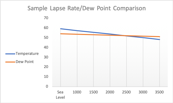
As you can see, there is a lot of theory in lapse rates. Dry lapse rate is essentially stable.. Moist lapse rate varies with conditions. The Standard Atmosphere Lapse Rate is pretty much “the average to use.” Here’s why it’s important.
In this example, we use the standard lapse rate of 3.6° and a dew point lapse rate of 1°.
The temperature at sea level is 59° with a dew point of 54°when the parcel of air begins to lift. As the elevation increases the dew point begins to drop by about 1° for each 1000 ft of elevation increase.
The temperature of the parcel lowers more quickly than the dew point.
Using 3.6° for each 1000 ft the temperature of the air parcel and the dew point within the parcel will equalize at about 2500 feet, resulting in condensation of the water vapor in the parcel.
Land warms and cools much quicker than nearby bodies of water. During the daytime, radiation from the sun creates warming of the land and the air above it. The resulting warmer air weighs less and begins to rise. A pressure gradient is formed between it and the cooler, denser air over the water, resulting in airflow from water to land. This effect is known as a sea breeze.
Typically a sea breeze will start up mid to late morning, build throughout the day, and die out late afternoon to early evening. With a classic sea breeze, as the wind increases in speed, it will veer. This means that a morning sea breeze from the west might veer to the northwest as the movement of air intensifies throughout the afternoon. As will be seen below, shape of the land can and does influence wind direction and veer.
Typically, a sea breeze is only felt a short distance offshore.
Image from weather.gov/jetstream/seabreeze
Warming land creates a warming of the air above it resulting in lower pressure.
The resulting pressure gradient moves the colder, denser air onshore.
A boundary between the colder air and the warmer air creates a small cold front which forces its way under the warmer air, causing it to rise
The rising air cools, resulting in a higher pressure area, generally 3,000 to 5,000 feet high.
The higher pressure air moves to fill in a lower pressure area over the ocean.
Sinking air results in a lower pressure area at 3,000 to 5,000 feet
The air higher pressure area resulting from the sinking air begins to move toward shore, completing and continuing the cycle.
Sea Breeze Channeling
A great example of a consistent, reliable sea breeze is found along the central coast of California around San Francisco. Throughout the summer, California’s interior valleys soak up the rays of the sun, often heating to 100 degree plus temperatures. The resulting low pressure allows to cooler heavier ocean air to move onshore beginning late in the morning.
As the breeze moves onshore, it runs into the Coastal Range of mountains, effectively blocking its movement. As with any fluid, the moving air seeks out the paths of least resistance. The most notable gap in the area is the Golden Gate, a 2 plus mile long, cliff lined channel through the land mass which narrows to less than 1 mile wide. The Golden Gate runs more or less southwest to northeast.
Consequently, the sea breeze from a large area of coastline is concentrated into a small area. The mild 5 or 10 knot sea breeze felt in the ocean off San Francisco is increased as it travels through the Golden Gate. By the time it reaches the bay, wind speeds are typically 25 or 30 knots, coming from the Southwest. From May to September, this process begins about 11:00 in the morning and generally dies out about 6:00 in the evening.
A similar effect on a larger scale is seen in the Strait of Juan de Fuca between Washington and Canada.
Land Breeze
A land breeze is essentially the reverse of a sea breeze. Land breezes only occur when the night time temperature of the land falls below the night time temperature of the sea’s surface. Land breezes are generally weaker than sea breezes.
Image from weather.gov/jetstream/seabreeze
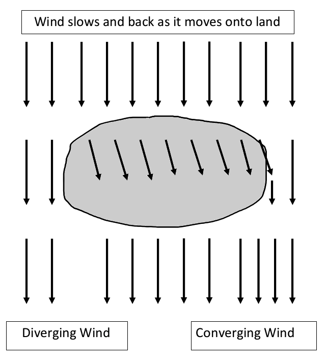
Wind speed and direction changes
In the northern hemisphere, wind veers as it speeds up and backs as it slows down.
Back over land – veer over water
When wind passes from water onto land, it slows down. As stated above, wind backs as it slows down. Therefore, you can expect wind to back as it passes from water onto land.
Conversely, wind passing from land onto water speeds up and therefore veers.
Convergence and Divergence
It is critical to note before we start this topic that this is a very limited aspect of convergence and divergence. We will only be looking at convergence and divergence on the surface, not the rising and sinking of air that also comes with it. This topic is covered in much greater detail and scope in the lessons on storms.
Convergence at the surface is wind from different directions coming together. More air in the same space results in faster airflow.
Divergence at the surface is wind separating and following different directions. Less air in a given area means slower wind speed.
Corner Effect
A corner effect is a small-scale convergence that can be quite severe. It occurs around steep islands and headlands.
Wind flowing over a low, flat island will slow and back. At the wind exits the island, it will tend to veer and speed up, however, with an area of divergence on the downwind right side of the island as it relates to the direction of wind flow, and an area of convergence on the downwind left side.
Wind Shadows
Any obstruction in the path of the wind creates a shadow where the wind is blocked or lessened for a distance on the leeward side of the object. What air flow that is present may be turbulent.
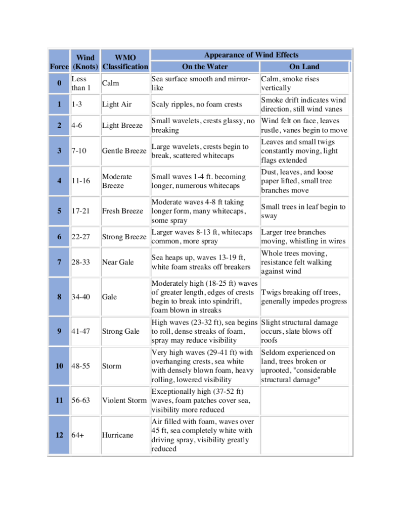
An anemometer is generally the best way to determine wind speed. However, when one is not available, you may determine the speed of the wind through the use of the Beaufort Scale.
A usable alternative
The Beaufort Scale allows you to use the appearance of the sea surface to estimate wind speed. The state of the sea, the dimensions of the waves, the presence of white caps, foam, or spray, depends principally on three factors:
Speed. The higher the speed of the wind, the greater is the disturbance.
Duration. Disturbance increases the longer the wind blows at a given speed, until a maximum state of disturbance is reached. In other words, the longer the wind blows, the bigger the waves get, to a certain point.
Fetch. This is the length of the stretch of water over which the wind acts on the sea surface from the same direction.
For a given wind speed and duration, the longer the fetch, the greater is the sea disturbance. If the fetch is short, such as a few miles, the disturbance is relatively small no matter how great the wind speed is or how long it has been blowing.
The Beaufort Wind Scale
The following table provides excellent guidelines on turning sea state observations into a usable estimate of wind speed.
Beaufort Wind Scale – Developed in 1805 by Sir Francis Beaufort, U.K. Royal Navy
In practice, the mariner observes the sea surface, noting the size of the waves, the white caps, spindrift, etc., and then finds the criterion which best describes the sea surface as observed.
A Caution
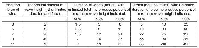
The Beaufort Scale assumes “steady-state” conditions. Rapid increases in wind speed take time to develop into sea state.
Duration and fetch
As can be seen in this table, Beaufort force 5 winds (17 to 21 kts) can develop into 8 foot wind waves. However, it requires over 8 hours and more than 60 miles of fetch to do so.
Significant wave height (SWH)
The maximum wave height in the second column is the average height of the highest one-third of the waves.
The first half of this lesson is a review of pressure gradient, Coriolis Effect, and wind speeds. For a more complete discussion refer to the High and Low Pressure Systems lesson.
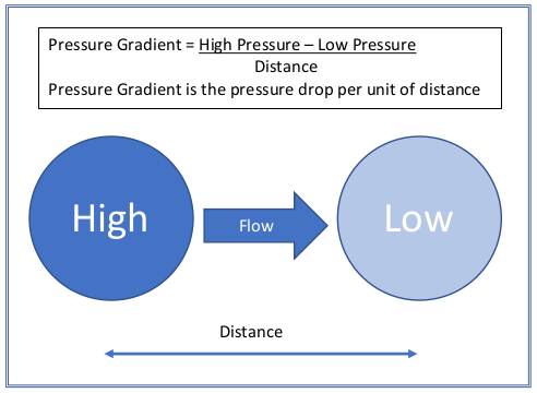
Pressure Gradient
Pressure gradient is the change in pressure measured across a given distance. Air flows from the high to the low because the pressure gradient creates a net force that starts the movement of air. The greater the pressure change over a given distance the greater the resulting net force, and the greater the air flow (wind).
Pressure Gradient
Air moves from high pressure to low pressure.
Coriolis Effect
As air moves from higher pressure into lower pressure, the Coriolis Effect causes the air to deflect, or turn to the right in the northern hemisphere and to the left in the southern hemisphere. The deflection is always in relationship to the air’s direction of travel. Unless otherwise stated, we will assume we are in the northern hemisphere.
A higher elevations, wind “starts” in same direction as the Pressure Gradient. The Coriolis Effect then turns the wind to the right, gradually moving further and further clockwise until the Pressure Gradient and the Coriolis Effect reach equilibrium with the air moving at 90° from the pressure gradient which is parallel to the isobars. In contrast, friction is counted in the equilibrium as the wind reaches the surface. The resulting wind does not make it quite 90°. The wind moves out of the high, but at about 15° to 30° across the isobars.
The closer the isobars, the higher the wind speed
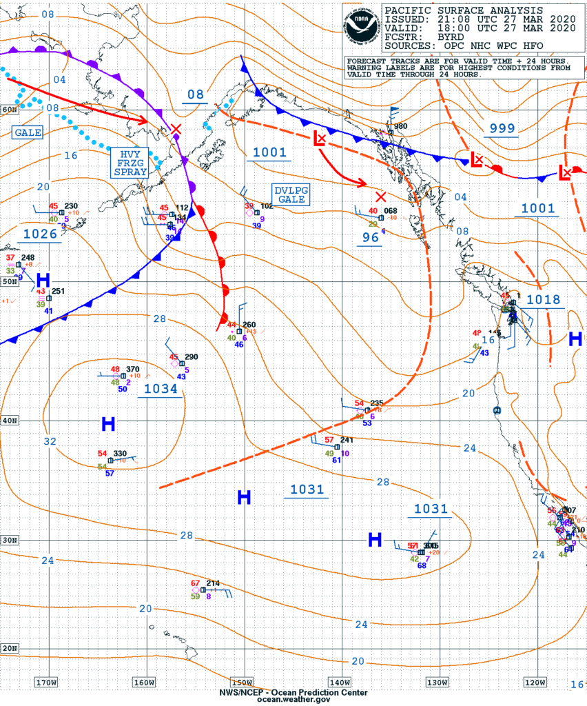
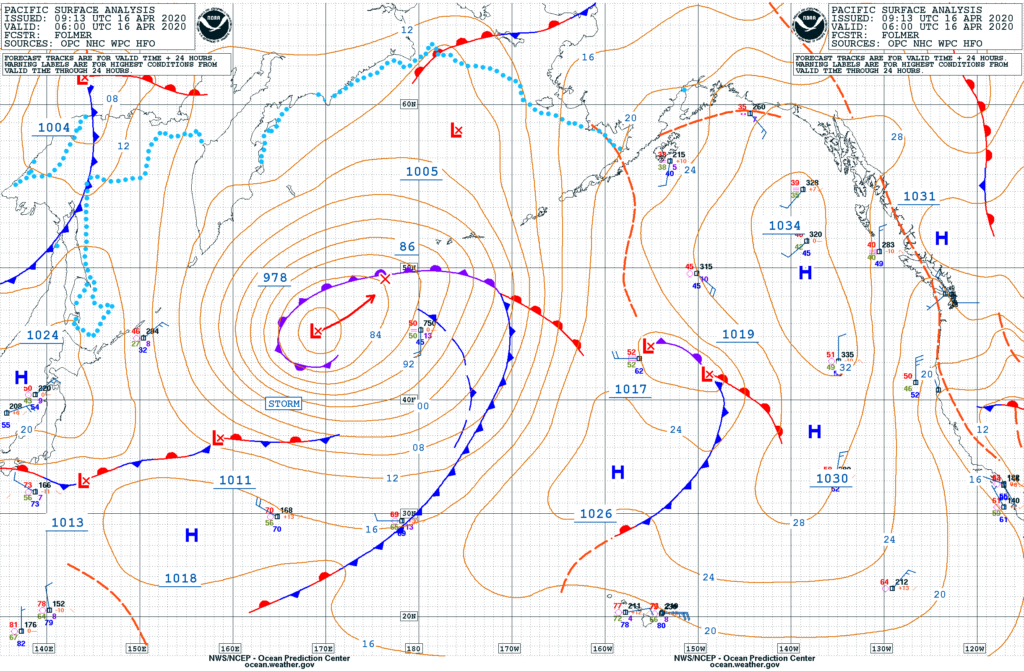
Pacific Surface Analysis 0600 UTC 16 April, 2020
The isobars are very close together near the low pressure system just to the left of center (Lat 40° N; Lon 165° E) in the above surface analysis. The closer together the isobars, the higher the pressure gradient, and the stronger the wind. At their closest point, the isobars measure about 1 apart. At that latitude, 1° isobar separation indicates winds of approximately 50 kts (see the table below). This estimate is verified by the STORM warning placed at the location. Storm force winds range from 48 knots (55 mph) to 63 knots (73 mph).
Calculating Wind From Isobars
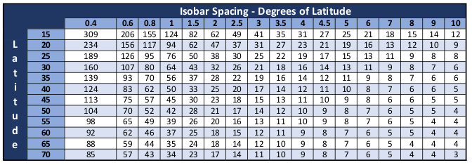
Measurement of isobar spacing provides a rough estimate of expected wind speeds. To use the table, measure the distance between isobars in degrees of latitude. Enter the table along the top row using that measurement. Find the closest latitude to the area of interest and follow that row. The intersection is the estimate of wind speed in knots.
Estimating Wind Direction
At upper altitudes, air flow is essentially parallel to the isobars. This knowledge is of little use to the sailor. Instead, wind direction at the surface is the concern. Remember that air flows clockwise around the highs and counterclockwise around the lows. It also flows out of the highs and into the lows. Consequently, if you measure the direction of the isobars and subtract 15° to 30° you have an approximate direction the wind is heading. For example; if the isobar direction is 180° at your location, expect the wind to be heading towards 150° to 165°. For simplicity, I would use 160°.
Conversely, add 15° to 30° when looking at air flow around a low.
Where is the wind coming from
It’s critical to understand that wind heading in the direction of 160° is coming from 340°. Wind is always labeled by its source, not its destination. This wind would be coming from the North Northwest (NNW), and would be labeled as such in any forecast.
Is there a simpler way
In practice, it is really quite simple. Lay a parallel ruler alongside the isobar. Rotate it 20 or so degrees out of the high or into the low and you have your wind direction.
Backing and Veering
Wind direction is constantly changing. When the wind changes direction to clockwise it is referred to as veering. It backs if it changes in a counter-clockwise direction.
Wind from 315 that shifts to 330 has veered. If it goes to 300 it has backed.
Apparent Wind vs. True Wind
True wind is the air movement you would feel if you are not moving. There are two dimensions to describing wind, speed and direction. For example, NW at 15kts, indicates wind coming from the northwest at 15 kts.
Apparent wind is the speed and direction wind seems to be coming from when you are moving. Thus, it is the sum of air movement and vessel movement.
Here is a visual. If you are stopped at a stoplight while riding a bicycle you feel true wind. Lets say that’s 5 kts of wind from directly in front of you. When you start moving, the wind will seem to increase with your speed. When you are moving at 5 kts, you will feel 10 kts of wind. At 10 kts, you feel 15 kts.
On the other hand, if the 5kts of wind is coming from behind, when you reach 5 kts of bike speed you will feel zero wind. At 10 kts of bike speed, you will feel 5 kts, and it will have changed direction to coming from the front.
A sailboat sails to the apparent wind.
Apparent wind is always forward of true wind
The movement of a vessel always rotates the apparent wind forward of the true wind in relation to the vessel. It the apparent wind is forward of the beam, apparent wind speed will be higher than true wind speed. If aft of the beam it will be less than true wind speed.
Plotting true or apparent wind
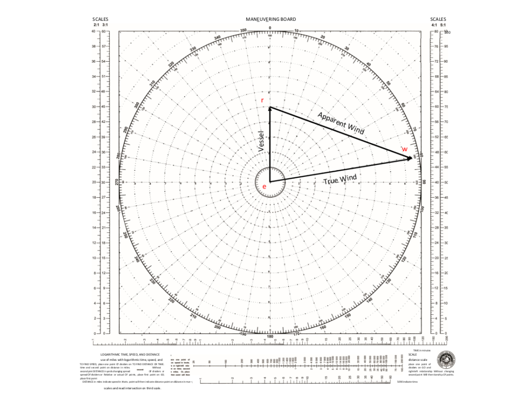
Vectors can be plotted on a Maneuvering Board to determine apparent wind or true wind the other is known.
Vessel course and speed are plotted first. In the example below, vessel is heading 360 at 5 kts. Point “e” is the vessel start point. Point “r” is the vessel location at end of a “one-hour” time.
If apparent wind is known, plot direction and speed beginning at point “r” and ending at point “w”. In the example, apparent wind is from 290 at 10 kts.
Plot the true wind vector “ew” to find the speed and direction of the true wind. True wind is from 261 (read off the inner degree scale) at about 9.5 kts.
If looking for what apparent wind to expect, plot the vessel’s vector, then the true wind. Relative wind can now be determined.
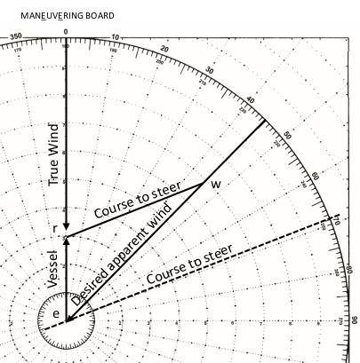
Course to steer to achieve desired apparent wind direction
The first thing you need. to know in order to determine course to steer is; “What is the closest my vessel will steer to the apparent wind?” For this example, let’s assume 45°.
First, assume your vessel is heading directly into the wind and draw vector ‘er’, your vessel, at 000. remember that “e” is generally located at the center of the plot.
Draw the 45° apparent wind vector that you would like to achieve. In this case you don’t know the speed, so draw the vector from “e” to the furthest edge of the plotting circle.
Set your dividers to the length of the wind speed. Scribe an arc centered on point “r”. The intersection of the apparent wind vector and the scribed arc is “w”. Vector “rw” is your course to steer in degrees “off” the wind. In this case, 069.
You may have noticed the Vessel course and true wind vectors are both on the 000 line. In practice, you may either show them both, or leave out the true wind vector. It isn’t needed in the calculation.
Now, apply the 069 course calculation to the actual true wind. If for example, the wind is from 315, steering a course of 246 puts you on a starboard tack with the apparent wind 45° off the bow. Conversely, a course of 024 results in a port tack with the same 45° apparent wind.
There are at least two formulas I know of to estimate wind speed based on spacing of isobars on a surface analysis. Both are based on the relationship between pressure gradient (e.g. millibars per degree) and the latitude of interest. For those that are interested, a discussion of each follows. Fortunately, it is much easier to use a table where someone else has done the math for you.
Estimated wind speeds based on surface analysis spacing of isobars. Assumes a spacing of 4mb per isobar. Wind speeds with tightly curved isobars may vary by up to 30%.
Calculating Wind Speed
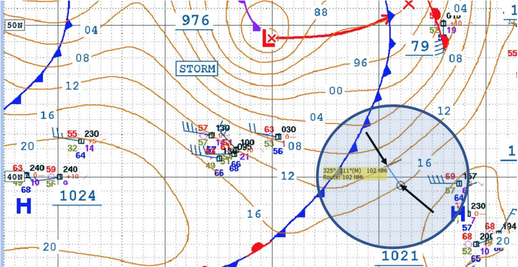
Measurement of the spacing of isobars can be done manually, or with the assistance of a tool. Here, a Surface Analysis of the Northeastern Pacific was loaded and displayed using OpenCPN, a chart plotter program. The shaded circle highlights the area of interest which is located on latitude 40.
Portion of a Surface Analysis. Isobar measurement completed with OpenCPN chart plotter program.
The two black arrows point to each end of a measurement tool. The yellow box indicates a measurement of 102nm. Divide 102 by 60 to get the the number of nautical miles in 1°. In the example, there are 1.7° between the two isobars, falling between two table columns. 40° latitude at 1.5 isobars/degree equals 33 kts winds. 2.0 isobars/degree equals 25 kts.
30 kts is a reasonable estimate of winds in the area.
Estimated Wind Direction
Estimate wind direction by looking at the direction of the isobars. Wind blows out of the high by 15° to 30° and into the low by the same. Interestingly, in both cases, subtract 15° to 30° from the direction of travel of the isobar for an estimate of wind direction.
Estimate wind direction in the example by taking the angle of the measurement (325°) and subtracting 90°. Resulting in the direction the isobar is coming from (235°). The wind travels into the low by an angle of 15° to 30°. Resulting in an estimated wind direction of 205° to 220°.
The title of this topic might have been “What causes the wind.” Quite simply, wind is moving air. Air doesn’t seem like much, however, it has weight and it has substance, and is actually considered a fluid. This becomes apparent when air moves. While moving, you can see many of the same characteristics you might find in a river. Things like moving as a “unit,” parting and coming back together as it flows around an obstacle, and eddies or back-flows.
Air moves from an area of higher pressure into an area of lower pressure. The closer together the high and low pressure is and the greater the difference in pressure, the faster the air flows.
Air has weight
The temptation is to believe air has no weight, which isn’t true. Logically, it must have weight. If not, you wouldn’t be able to feel the wind on your face while sailing, and your sails would hang limp even in a fresh breeze.
An Interesting Example
On August 16, 1960, Air Force Captain Joseph Kittinger made a high-altitude parachute jump from 102,800 feet (nearly 20 miles high). At that altitude there is so little air pressure, and so few air molecules, that there was no impression of falling. Moving at a speed of 614 mph, Kittinger’s flight suit did not even flap in the “wind” because there was insufficient air molecules and weight to move the fabric.
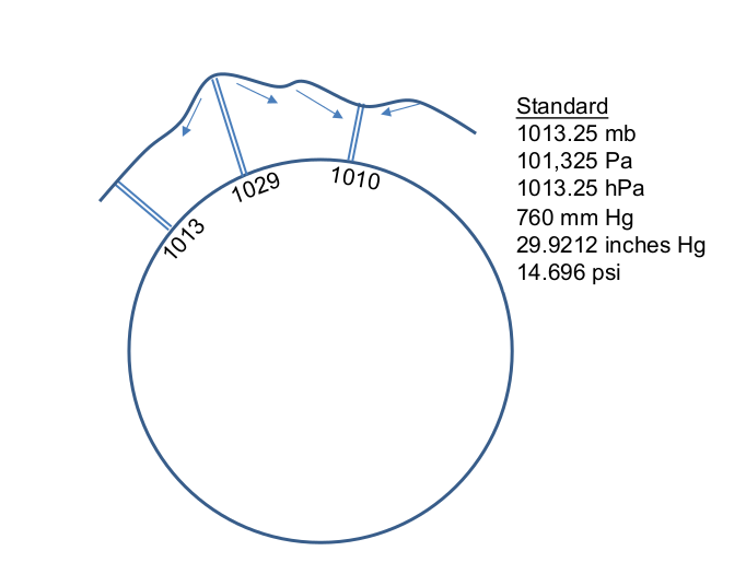
Standard Atmospheric Pressure
If you weigh the column of air directly above you, it would weigh approximately 14.696 pounds per square inch. This is also known as the standard atmospheric pressure. As the graphic demonstrates, there are a number of labels to use when expressing standard pressure. All represent the same value.
Weight of a column of air
Millibars
In the maritime world, millibars (mb) are used. Standard pressure in millibars is 1013.25(mb). Throughout these lessons, we will be using millibars to express atmospheric pressure, however, you may have occasion to check weather briefings and forecasts that use other units of measurement. For example, aviation forecasts typically use inches of Mercury (Hg), where standard pressure is 29.9212 inches (Hg).
Atmospheric pressure is also known as barometric pressure.
In the Island in the Sun analogy in Convection Cells and Global Weather Patterns, heated air ascended, traveling away from where it rose it was added to the “pile” of air at another location, creating a higher pressure at the new location. There are other ways in increase atmospheric pressure in a given area. For example, cold air is heavier the warm air. Moisture laden air is heavier than dry air. Consequently, all of these factors are added together to determine pressure in a given area.
High Pressure vs. Low Pressure
Relatively small variations in pressure determine the wind and storm patterns around the world. The highest pressure every recorded was 1083.98 mb at a location in Siberia. Whereas the lowest, 877.07, occurred in the eye of a South Pacific typhoon. In contrast, most readings fall between 975 mb and 1050 mb, a pressure difference that can easily result in wind speeds in excess of 50 kts!
Pressure Gradient
Pressure gradient is the change in pressure measured across a given distance. Air flows from the high to the low because the pressure gradient creates a net force that starts the movement of air. The greater the pressure change over a given distance the greater the net force, the greater the air flow.
Pressure Gradient
Air moves from high pressure to low pressure.
Coriolis Effect
Air moves from higher pressure into lower pressure, however, not in a straight line as demonstrated above. Instead, something called the Coriolis Effect causes the air to deflect, or turn.
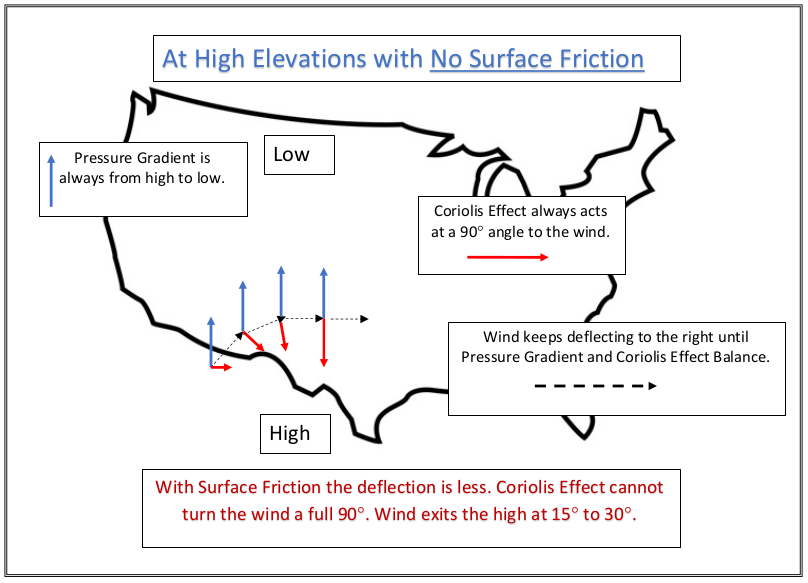
At higher elevations, with no surface friction, the Coriolis Effect turns the wind 90 degrees to the right.
The Coriolis Effect works at 90° to the wind
The wind starts in the same direction as the pressure gradient. The Coriolis Effect working at 90° to the right causes the wind to change direction so that it balances the two forces. The Coriolis Effect will now start working at a 90° angle to the new wind, forcing the wind to turn further. Again, the Coriolis Effect works at 90° to the wind, forcing it to turn further. This process continues until the pressure gradient and the Coriolis Effect balance each other out.
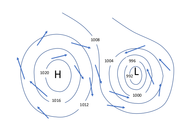
The Coriolis Effect describes the bending of the trajectory of an object as it travels. In the Northern Hemisphere, air that is moving out of a high pressure system towards an area of lower pressure bends to the right. In the Southern Hemisphere the effect is the opposite, bending flow to the left.
Wind “starts” in same direction as Pressure Gradient. The Coriolis Effect turns the wind to the right, gradually moving further and further clockwise until the Pressure Gradient and the Coriolis Effect reach equilibrium. At the surface, friction is counted in the equilibrium, resulting the the wind moving out of the high at about 15° to 30° instead of getting parallel to the isobars.
Air flows from higher to lower pressure. Add in the Coriolis Effect caused by the Earth’s rotation and the air flows clockwise (in the northern hemisphere) around and out of a high pressure system into the lower pressure where it rotates counter clockwise.
Clockwise Around the High
Here’s some good news. Unless you are a scientist or a mathematician, all the details really doesn’t matter to the typical sailor? Just remember, in the northern hemisphere high pressure systems rotate clockwise and low pressure systems rotate counter clockwise. The wind travels slightly out of the highs and slightly into the lows.
The opposite is true in the southern hemisphere.
Around and Out
We now know the net force resulting from the pressure gradient gets the air moving out of the high, towards the low. Once moving, the Coriolis Effect begins to turn the moving air to the right. The air continues deflecting to the right until the net force of the pressure gradient and the turning force of the Coriolis Effect balance each other out. As a result, the air flows clockwise around and out of the high by 15° to 30°. The same effect causes air entering a low to turn to the right, moving counter-clockwise around the low.
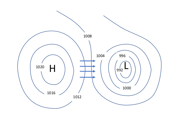
Isobars
Isobars are the contour lines of atmospheric pressure. They are a series of lines on a map connecting points having the same atmospheric pressure. Each isobar is labeled with its represented pressure, generally with a four millibar spacing.
Surface Analysis covering the North-eastern Pacific valid as of 1800 UTC on March 27, 2020.
In this surface analysis forecast example, a high pressure area can be seen on the left side of the image, slightly below center at latitude 40N. The “H” indicates the center of the high. The expected high pressure there is 1034mb. It’s important to note the “1034” label is underlined, and is not found at the actually location of the highest pressure. In this case, it is slightly above and to the right. The first isobar out from the “H” is 1032mb and includes just the last two digits of the pressure (32). Each successive isobar is 4mb less than the one before; 28, 24, 20, etc.
Moving to the upper right on the map, is a low pressure area with an atmospheric pressure of 999 in the position of the X next to the “L”. Although not marked, the small circle surrounding the “Lx” represents a pressure of 1000 isobars. Take a moment to locate and identify the pressure for each isobar between the areas of high pressure and low pressure.
Properties of Highs and Lows
Calculating Wind from Isobars by Table Lookup
There are at least two formulas I know of to estimate wind speed based on spacing of isobars on a surface analysis. Both are based on the relationship between pressure gradient (e.g. millibars per degree) and the latitude of interest. For those that are interested, a discussion of each follows. Fortunately, it is much easier to use a table where someone else has done the math for you.
Estimated wind speeds based on surface analysis spacing of isobars. Assumes a spacing of 4mb per isobar. Wind speeds with tightly curved isobars may vary by up to 30%.
Calculating Wind Speed
Measurement of the spacing of isobars can be done manually, or with the assistance of a tool. Here, a Surface Analysis of the Northeastern Pacific was loaded and displayed using OpenCPN, a chart plotter program. The shaded circle highlights the area of interest which is located on latitude 40.
The two black arrows point to each end of a measurement tool. The yellow box indicates a measurement of 102nm. Divide 102 by 60 to get the the number of nautical miles in 1°. In the example, there are 1.7° between the two isobars, falling between two table columns. 40° latitude at 1.5 isobars/degree equals 33 kts winds. 2.0 isobars/degree equals 25 kts.
30 kts is a reasonable estimate of winds in the area.
Estimated Wind Direction
Estimate wind direction by looking at the direction of the isobar. Wind blows out of the high by 15° to 30° and into the low by the same. Interestingly, in both cases, subtract 15° to 30° from the direction of travel of the isobar for an estimate of wind direction.
Estimate wind direction in the example by taking the angle of the measurement (325°) and subtracting 90°. Resulting in the direction the isobar is coming from (235°). The wind travels into the low by an angle of 15° to 30°. Resulting in an estimated wind direction of 205° to 220°.
Portion of a Surface Analysis. Isobar measurement completed with OpenCPN chart plotter program.
Elevation and adjusting to “sea-level”
As you move higher in the atmosphere, there are fewer air molecules above you. Consequently, there is less weight, meaning less air pressure. Beginning at sea level, the first 1000 feet will result in a pressure change of about 36 mb. As a result, assuming a sea level pressure of 1013.25 mb, someone at 10000 feet would be experiencing only 696.82 mb. It’s easy to see how this presents a problem if displayed that way on a weather map. Owing to this, all air pressure measurements are adjusted to their sea level equivalent before use.
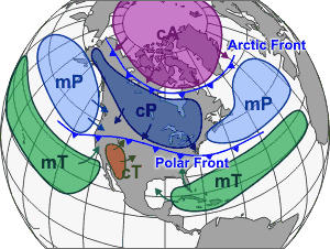
An air mass is a large volume of air defined by two basic factors. What is the moisture content and is the air warm or cold. As a result, air masses are typically broken into five basic types.
North American Air Masses from weather.gov
Moisture Content
Moisture content is the primary defining characteristic. Air is either Continental (c) or Maritime (m). Continental air masses form over dry land and consequently have little moisture content. Maritime air masses on the other hand, form over oceans and are therefore moist.
Temperature
Each of these air mass types are then further divided by the temperature of the area they are formed.
Tropical (T) air masses form in the warm lower latitudes and are consequently warm in nature.
Polar (P) air masses originate in cold higher latitudes.
Arctic (A) air masses start out in the arctic and antarctic areas with results in extremely cold air.
The five basic air mass types
Combining these two basic air mass characteristics together results in five basic types.
mT – Warm moist air. Formed over the oceans in lower latitudes.
mP – Cold moist air. Formed over the oceans in higher latitudes.
cT – Warm dry air. Formed over land in lower latitudes.
cP – Cold dry air. Formed over land in higher latitudes.
cA – Very cold dry air. Air is so cold in this area that it is not able to sustain any kind of moisture content. As a result, there is no maritime arctic classification.
These five basic air mass types may be further broken down by specific areas, such as “equatorial” or “monsoon”, however, it isn’t needed as part of basic marine weather knowledge.
Air masses don’t appear to form as much in the middle latitudes. Instead, the mid latitudes seem to be dominated by the movement of air masses from higher and lower latitude areas.
After formation air masses move around. Air mass movement is controlled by air flow in the upper atmosphere. As an air mass moves into a new area, it may pick up characteristics from the new area. Arctic air moving south into Canada may warm but will stay dry. That same air mass moving south over the Pacific Ocean not only warms, it picks up moisture, possibly changing enough to become a maritime polar (mP) air mass.
An introduction to fronts
The boundary where two air masses converge is known as a front. Later, we will be spending a good amount of time exploring different types of fronts and their associated weather patterns. For now, we focus on just a couple of main types.
Cold fronts and warm fronts
A cold front is a colder air mass replacing a warmer air mass.
A warm front is the opposite affect. Warm air replacing cold air.
There is also a stationary front where the boundary between two air masses does not move.
Pacific Surface Analysis 0600 UTC 16 April, 2020
All four primary front types can be seen in this weather map. Cold fronts are identified with a blue line and blue triangles. The direction the triangle points is the direction of movement of the front. Warm fronts are indicated by red lines with red half circles in the direction of front movement.
There is a great example of a stationary front in the lower left portion of the map (running along latitude 33 to 37). There is a cold front from the north and a warm front from the south. The front boundary is marked with a line with alternates blue and red, as well as triangles and half circles.
Occluded fronts are indicated by a purple line with alternating triangles and semicircles. Again, this surface analysis has a great example at 50N, 170E.
Weather is based on the relationship of the Sun to the Earth.
Hadley Cells
As seen in “Island in the Sun”, the rays of the sun heat the earth and the air above it. The more directly the rays of the sun impact the Earth, the more energy is transferred heating the Earth and the atmosphere above it.
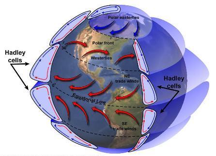
The sun is located more or less over the equator. Because of this, the air near the equator is heated more causing it to rise vertically.
Heated air from the equator begins to move toward the poles and to cool. As the air cools, it begins to descend back to the Earth’s surface. The cooling air descends about latitude 30, causing a “pile” of extra air to end up at that location. This results in an area of higher pressure. Then, as the cooled air reaches the Earth’s surface it heads back to the equator. Filling in for the air that is heated and rising air.
Hadley cells are the basis for our understanding of global-scale meteorology. Image by NASA
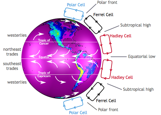
The Hadley cell forms a convection cell dominating lower latitude (0° to 30°) tropical and sub-tropical climates. Two other convection cells join, the Hadley Cell setting global circulation patterns into motion.
Polar Cell
The air at the poles is much colder than the air around latitude 60. Meaning, the air rises from around latitude 60 and travels toward the poles. Once over the poles, it sinks, forming the polar highs. At the surface air diverges out and away from the pole, back to latitude 60. The resulting convection cell is referred to as a Polar Cell
Kind of the same
In many ways, Hadley Cells and Polar Cells are similar. In both cases, air rises from a warmer location, travels north towards the pole, sinks, and finally travels away from the pole to its starting point. Convection cell rotation with both is the same direction.
In contrast, between the two is a cell rotating in the opposite direction.
Ferrel Cell
The sinking air from the Hadley Cell (near latitude 30) drags air beside it down, while air rising in the Polar Cell (about latitude 60) takes nearby air up with it. The rising air then moves away from the pole at high altitude. The opposite the direction of the other cells. On the other hand, the sinking air moves toward the pole along the surface of the Earth.
Another look at the three types of convection cells. Image by the Center for Multiscale modeling of Atmospheric Processes.
Global Wind Belts
As described in the video, there are three global wind belts north, and three south of the equator. Located close to the equator are the Trade Winds (also known as the Tropical Easterlies), blowing from east to west. Located from around 30° to 60°are the Prevailing Westerlies. Finally, north and south of 60° are the Polar Easterlies.
Bands of High and Low Pressure
A band of high pressure lies between the Hadley cells and Ferrel Cells. The high-pressure band is located about 30° North and South latitude. Each pole is the location of another high pressure area.
The equator and 50° to 60° North and South latitude are low pressure bands.
Associate hot, dry weather with high pressure. In contrast, rainy and stormy weather is associated with low pressure. The regions between 50° and 60° tend to have more precipitation due to more storms moving around the earth at these latitudes, especially along the west coast of continents. While many of the Earth’s desert areas are located along latitude 30°. Also, large high pressure areas are found in the middle of oceans at that latitude.
We look at high and low pressure, and the properties of each in a later lesson.
Seasonal Changes
One final topic before closing this lesson. The axis of the Earth does not sit straight up and down. It tilts in relationship to the sun at approximately 23.44°.
Due to the tilt of the Earth, the sun is directly over the equator only twice a year, on about March 20th and September 22nd. During the summer and winter, the sun slowly “moves” north and south of the equator to a maximum of 23.44° north on about June 21, and 23.44° south on about December 21 . The maximum latitude marking the sun’s location is known as the Tropic of Cancer in the north, and the Tropic of Capricorn in the south. The “tropics” lie between Tropic of Cancer and Tropic of Capricorn.
As the sun moves north and south of the equator, Hadley Cells and Ferrel Cells, as well as their associated high and low pressure systems move also. The perfect example is the semi-permanent North Pacific High. Centered about 30° north, the North Pacific High moves north in the summer to roughly 38°.
Watching this video demonstrates what happens by tracking water vapor in the atmosphere over the course of a year. Watch the top of South America. At the beginning and end of the video (winter time), the vapor trail is much lower than during the summer in the middle.
A vector is any quantity, such as a force, velocity, or acceleration, which has both magnitude and direction. Such a quantity may be represented geometrically by a plotted line or arrow of a length proportional to its magnitude which is pointing in the given direction.
Course and speed of a vessel when taken together represent a vector.
Direction and speed of wind is a vector
On a plotting sheet vectors used in navigation and weather are labeled with standard notations.
er = speed and direction of your vessel
rw = relative wind (aka apparent wind)
ew = true wind
Vector (line) er goes from point “e” (beginning location of your vessel) to point “r” (end location of your vessel).