CPA – Closest Point of Approach

Why?

Radar Screen Orientation

The first thing to know is how your radar is set to display. Head Up, North Up, or Course Up. There are pro’s and con’s to each setting, and it really comes down to what your personal preference is.

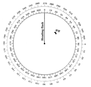
Head Up

Head up always orients the screen to the direction your vessel is heading. Your direction of travel becomes 000. I see two main benefits to Head Up. First, all target echos are exactly relative to your vessel. Assuming clear visibility, if the screen paints a target at 090, all you need to do is look directly off the starboard beam. The target will be there. Second, when plotting own vessels course you will always plot directly on the 000/180 line (more on that in the Determining Other Vessel Course and Speed).

The disadvantage is an additional calculation when determining the other vessel’s true course. Again, more to come on that topic.

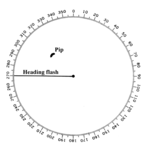
North Up

North Up uses a direction sensor to orient your screen to north. 000 on the screen will represent North, and a heading flasher (line) will appear to show your vessel’s heading. North Up takes a relative bearing and rotates it in such a way it is lined up with North. For example, if you are on a course of 045, a relative bearing of 090 degrees will paint on the screen at 135 degrees. Meaning that an object directly off the starboard beam may appear to be behind you while looking at the screen. On the other hand, using a compass oriented at 135 (don’t forget to adjust for variation) will point you in the direction of the object. While plotting your own course on the maneuvering board while in North Up mode, remember to plot using the direction of your heading, not the 000/180 line.

The primary advantage of North Up comes later, while calculating the other vessel’s true course.

Course Up

Course up is essentially the same as head up until you execute a turn. It will generally be treated in the same way as head up mode while calculating CPA and Time to CPA.

Plotting Relative Contact Locations

Knowing your screen’s orientation is important, however, it does not impact the “how to” of finding CPA. Simply plot what you see on the screen. For the purpose of this discussion, we will be assuming exercises have the display set to head up.

Relative Bearings

As it pertains to radar, a relative bearing is always in relationship to your vessel’s heading, and progresses clockwise from 000° to 360°. Notation for a relative bearing is as follows: 045R is 45° clockwise of your vessel’s heading. 270R is 270° clockwise from the heading. A radar bearing is never cited as counter clockwise (left of) your current heading. A more complete discussion of True, Magnetic, and Relative bearings can be found in the Bearings lesson.

Relative Plot

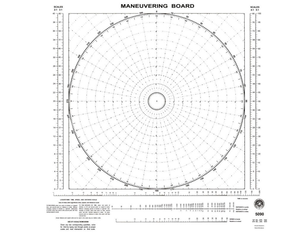
To determine CPA, first create a relative plot showing the movement of your vessel vs the other vessel. A maneuvering board is a good tool for this task. An 8.5 x 11 inch pdf of a maneuvering board can be downloaded from the link at the top of the page. Various items within the plot must be labeled to prevent confusion and to help ensure success. There are a couple of different labeling methods in use. The one presented here is the one most commonly used. A second set of “vector triangle” labels used to identify relative to true vectors and course to steer vectors will be introduced later.

Relative Plot Labels

• R … Your Ship
• M … Other Ship
• M₁ … First Plotted Position of Other Ship
• M₂, M₃ … Later Plotted Positions of Other Ship
• M_x … Planned Position of Other ship at time of your maneuver to avoid
• Note: If more than one vessel is being tracked, replace M with another letter such as N, O, P, etc.

• RML … Relative Motion Line
• DRM … Direction of Relative Motion
• SRM … Speed of Relative Motion
• MRM … Miles of Relative Motion
• NRML … New Relative Motion Line

• CPA … Closest Point of Approach

Plotting the Target’s Location

When a target first appears on the radar, use the VRM and EBL tools to determine range and bearing. On a maneuvering board, plot the range and bearing of the target, as well as the time and a target identifier. In this case the target will be identified as “M”. The first plotted location will be identified as M₁.

Every plotted location has 4 data points:

1. Target “Name” (M, N, O …)
2. Time
3. Range
4. Bearing

Allow a period of time to elapse and use the VRM and EBL tools to capture the new range and bearing to the target. A common time lapse between plots is 6 minutes, although any convenient length of time may be used.

Plot this second location on the maneuvering board and label as M₂. While it’s desirable to have at least three plotted locations to ensure accuracy, two plotted locations can be used to begin an examination of the possibility of collision between you and the target.

6 Minute Rule

6 minutes is a standard time lapse between target plots because the distance traveled in 6 minutes is 1/10 of the speed. For example, if a vessel traveled .7 miles over 6 minute period of time that vessel speed is 7 knots.

RML (SRM & DRM)

Once you have two or more target locations plotted take a straight edge and draw a line beginning at M1 through M2 and continuing until you have gone past the center of the maneuvering board. Remember, that the center represents your vessel’s location.

This is your relative motion line and should be labeled RML. The direction of the RML in degrees is the direction of relative motion (DRM). It can be helpful to draw an arrow head at the end of the RML to remind you of the relative direction of travel between you and the other vessel. During later steps, it can be easy to confuse the DRM and use its reciprocal.

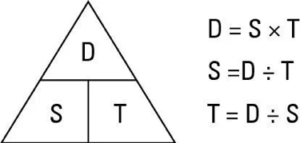
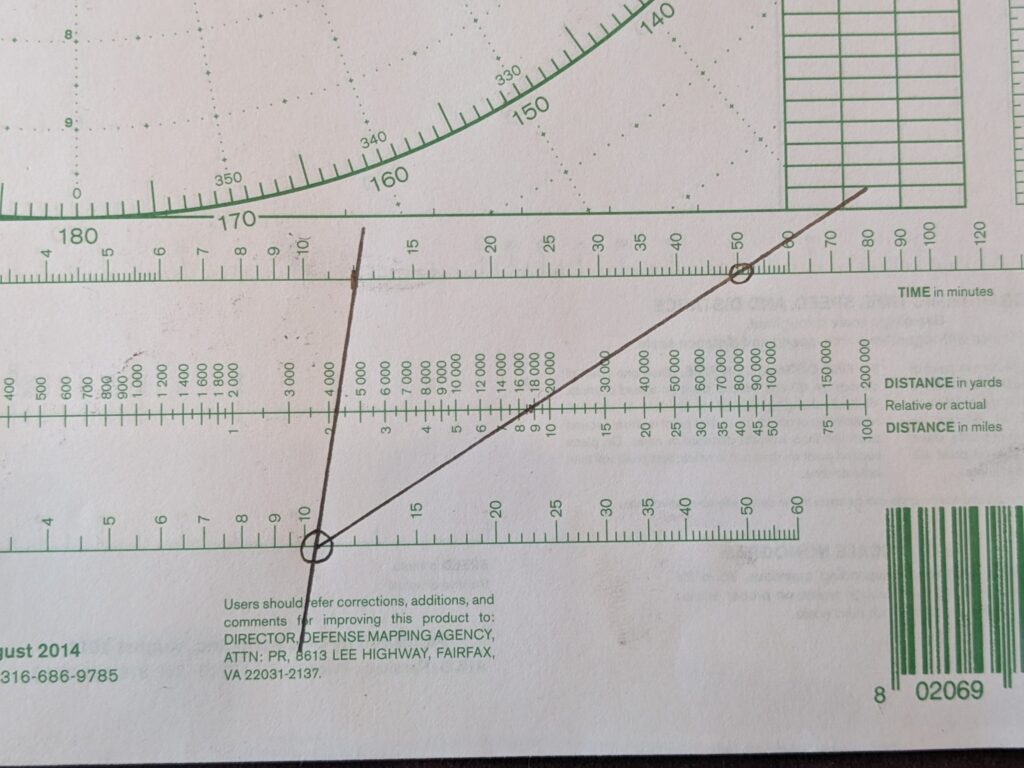
Measuring the distance between M₁ and M₂ provides the speed of relative motion (SRM). If you are using the 6 minute rule, simply multiply the distance traveled between M₁ and M₂ by 10. If any other time span is used, the nomogram at the bottom of the maneuvering board or “D Street” will assist in getting the correct speed.

The D Street Triangle

If RML crosses directly through the center you are on a collision course. If it passes above or below the center, you are not and it’s time to calculate how close the vessel will be to you at its closest point of approach as well as what time that will happen.

An example

• M₁ at 0900 indicates a range of 9.0nm with a bearing of 274R
• M₂ at 0906, 8nm, 276R
• M₃ at 0912, 6.9nm 278R

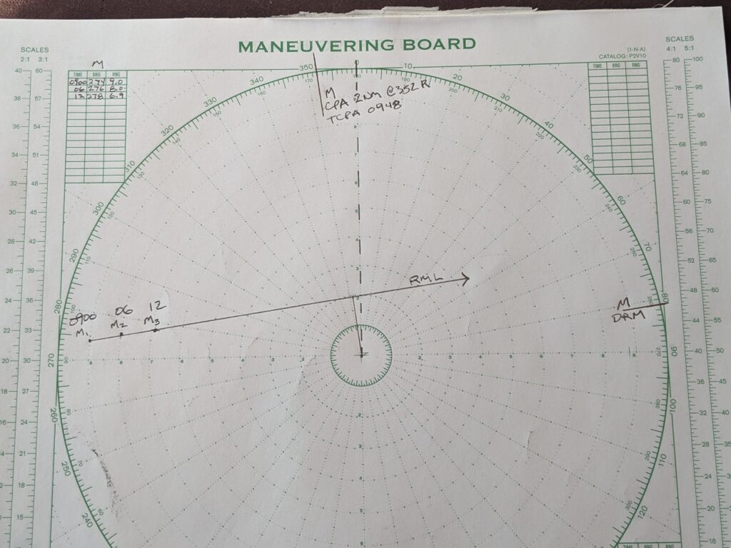
Once drawn, the RML is “moved” to the center and the bearing check against the compass scale. Other ship “M” has a DRM of 081R.

SRM is found by measuring the distance between any two plotted points along the RML. Two different ways to find the solution are provided. The measured distance from M₁ to M₂ is 1.1nm. Applying the 6 minute rule provides a SRM of 11 knots. In the image on the right, the nomogram is used to calculate SRM from M₁ to M₃, a distance of 2.2nm over 12 minutes. The top scale of the nomogram is time in minutes. The middle scale is distance in yards and/or miles. The bottom scale is speed. Drawing a line from 12 minutes thru 2.2 miles provides a speed solution of 11 knots.

Finding the CPA (Direction and Distance)

One the RML has been plotted it becomes easy to determine the closest point of approach distance, direction, and time. Scribe a line perpendicular to the RML from the center to find direction. The distance from the center to the RML provides distance. In the image above, CPA will be approximately 2nm at 352R (8^∘ to port looking over the bow).

Time to CPA (TCPA)

Time to CPA in the example is 48 minutes from point of first contact. It is a simple process to measure the distance from the plotted contact to the CPA. In this case, 8.8 miles from M₁ to CPA. Using the 11 knot relative speed calculated earlier, TCPA is 48 minutes (8.8 / 11 = .8 hours or 48 minutes). First contact was 0900. TCPA would be 0948.

Using the nomogram provides approximately the same answer as illustrated above.

Testing Your Skills

Here are two additional CPA problems. Plot the contacts and determine:

• DRM
• SRM
• Direction to CPA
• Distance to CPA
• TCPA